Single Cell RNA-Seq

In this tutorial we are going to run through how UCDeconvolve can be used to aid in the analysis and annotation of single-cell RNA-Sequencing data. For this tutorial, we are going to use the ‘pbmc3k’ dataset provided in the scanpy datasets model at sc.datasets.pbmc3k().

Loading Packages & Authenticating

The first step in this analysis will be to load scanpy and ucdeconvolve after following the installation and registration instructions, and authenticate our API. In this tutorial we saved our user access token in the variable TOKEN.

import scanpy as sc
import ucdeconvolve as ucd

ucd.api.authenticate(TOKEN)

2023-04-25 15:57:57,357|[UCD]|INFO: Updated valid user access token.

| .. note:: By default the logging level is set to DEBUG. To change logging levels you can import logging and set ucd.settings.verbosity directly. To reduce logs, change verbosity to logging.INFO. In general we recommend keeping logging to DEBUG to provide status updates on a running deconvolution job.

Loading & Preprocessing Data

We will now begin by loading our pbmc dataset.

adata = sc.datasets.pbmc3k()

We will save raw counts data into adata, which can serve as an input to ucd functions. Unicell will detect non-logarithmized counts data and automatically normalize our data. We will run a quick built-in preprocssing functions using scanpy to obtain some clustered data. This step will take a minute or two to complete.

adata.raw = adata

sc.pp.recipe_seurat(adata)

sc.tl.pca(adata)
sc.pp.neighbors(adata, n_neighbors = 30)
sc.tl.umap(adata, min_dist = 0.1)
sc.tl.leiden(adata, resolution = 0.75)

We plot the UMAP of our dataset using leiden clusters as an overlay and see the following image:

sc.pl.umap(adata, color = 'leiden')

Initial Cluster Identification Using UCDBase

To get a general sense of the celltypes most likely present in this dataset, we want to first run ucd.tl.base which will return context-free deconvolutions of cell type states.

ucd.tl.base(adata)

2023-04-25 13:10:28,425|[UCD]|INFO: Starting UCDeconvolveBASE Run. | Timer Started.
Preprocessing Dataset | 100% (11 of 11) || Elapsed Time: 0:00:01 Time:  0:00:01
2023-04-25 13:10:30,501|[UCD]|INFO: Uploading Data | Timer Started.
2023-04-25 13:10:31,339|[UCD]|INFO: Upload Complete | Elapsed Time: 0.838 (s)
Waiting For Submission : UNKNOWN | Queue Size : 0 | / |#| 0 Elapsed Time: 0:00:00
Waiting For Submission : QUEUED | Queue Size : 1 | | |#| 3 Elapsed Time: 0:00:04
Waiting For Submission : RUNNING | Queue Size : 1 | / |#| 3 Elapsed Time: 0:00:04
Waiting For Completion | 100% (2700 of 2700) || Elapsed Time: 0:00:28 Time:  0:00:28
2023-04-25 13:11:07,163|[UCD]|INFO: Download Results | Timer Started.
2023-04-25 13:11:08,505|[UCD]|INFO: Download Complete | Elapsed Time: 1.342 (s)
2023-04-25 13:11:09,238|[UCD]|INFO: Run Complete | Elapsed Time: 40.812 (s)

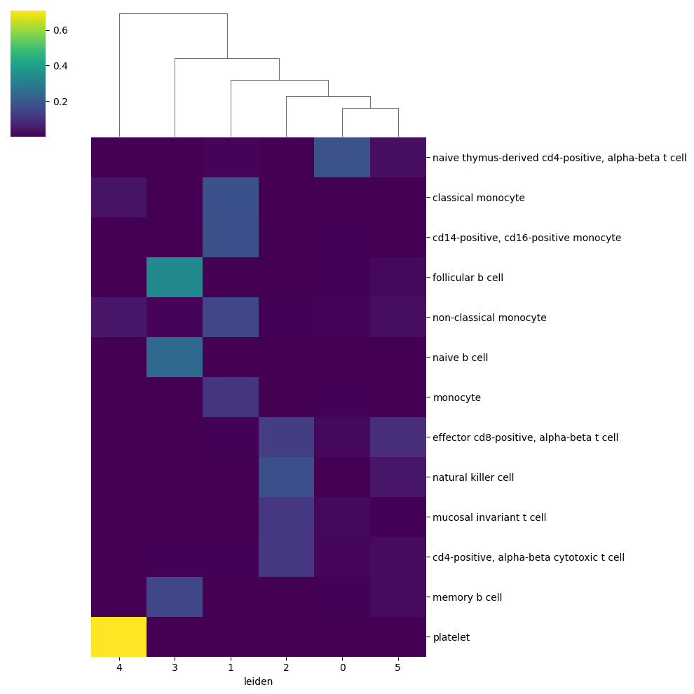
Plotting Clustermap

To get a general sense of the deconvolution results, let’s plot a clustermap that aggregates base predictions on the basis of leiden cluster using the function ucd.pl.base_clustermap

ucd.pl.base_clustermap(adata, groupby = 'leiden', n_top_celltypes=75)

<seaborn.matrix.ClusterGrid at 0x16b06d430>

We can see that the predictions shown in the clustermap are hierarchecal. By default, ucdeconvolve base performs belief propagation, which takes flattened predictions and aggregates them up a cell type heirarchy. This flag can be set in the ucd.tl.base function as propagate = False. For most cases we reccomend peforming belief propagation, as it accounts for uncertainty in ground-truth labels used during training.

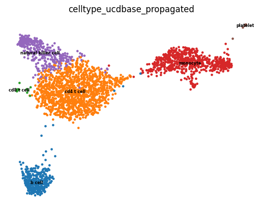
In either case, we can use this clustering information to label our dataset by selecting the most likely detailed cell subtype, using ucdbase to guide us to an answer faster than performing manual curation.

label = "celltype_ucdbase_propagated"
adata.obs[label] = 'unknown'
adata.obs.loc[adata.obs.leiden.isin(("1",)), label] = "monocyte"
adata.obs.loc[adata.obs.leiden.isin(("4",)), label] = "platelet"
adata.obs.loc[adata.obs.leiden.isin(("3",)), label] = "b cell"
adata.obs.loc[adata.obs.leiden.isin(("0",)), label] = "cd4 t cell"
adata.obs.loc[adata.obs.leiden.isin(("2",)), label] = "natural killer cell"
adata.obs.loc[adata.obs.leiden.isin(("5",)), label] = "cd8 t cell"

sc.pl.umap(adata, color = 'celltype_ucdbase_propagated', legend_loc = 'on data',
           legend_fontsize = "xx-small", frameon = False)

Examining Feature Attributions with UCDExplain

To gain some additional insight into the cell types being predicted for each cluster, we can leveraged integrated gradients which is implemented in the ucd.tl.explain module. This method takes a target output for the ucdbase model and computes attribution scores for all input genes. A positive attribution score indicates that a given gene’s expression is positively associated with the prediction of that given cell type (i.e. canonical marker genes tend to have high feature attribution scores for their corresponding cell types) while a negative attribution score indicates that a given gene’s expression is negatively associated with the prediction of that given cell type (i.e. it may be a canonical marker of another cell type). We can use feature attributions to validate some of our predictions by confirming that the top genes associated with a given cell type are concordant with biological phenomena.

Examining Raw Predictions

To do this, we first must examine the models raw, non-propagated predictiosn. As feature attributions using integrated gradients relies on the core wieghts underpinning the ucdbase deep learning model, it does not consider belief propagation which is a post-processing function. Therefore, we ned to first get a sense of the “raw” cell type predictions made for each cluster.

We can plot raw cell type predictions using the same clustermap function above, but this time adding an additional parameter.

ucd.pl.base_clustermap(adata, groupby = 'leiden', category = 'raw', n_top_celltypes = 75)

<seaborn.matrix.ClusterGrid at 0x16b0c27f0>

We can immediately see that these predictions are alot more specific for each cluster. We include a utility function to assign target cell types from predictions to each cluster, and can use this ‘raw’ prediction information to collect feature attributions for each cluster individually. This functions creates a new column in adata.obs entitled pred_celltype_{key} which in our case key, which represents the name of the run call, defaults to ucdbase, therefore our column is called pred_celltype_ucdbase.

ucd.utils.assign_top_celltypes(adata, category = "raw", groupby = "leiden")

Let’s plot the resulting ‘raw’ assigned celltypes over our UMAP and compre them with our aggregated propagation assignments we performed semi-manually.

sc.pl.umap(adata, color = ["pred_celltype_ucdbase", "celltype_ucdbase_propagated"],
           legend_loc = 'on data', legend_fontsize = 'xx-small', frameon = False)

Running UCDExplain

Warning

As feature attributions is a highly computationally intensive operation, for scRNA-Seq data where each cell is considered a sample, we highly recommend utilizing the subsampling capabilities built into ucd.tl.explain to speed up peformance. When run at the cluster-level, we find that subsampling a sufficient number of cells from each cluster provides the same level of feature attribution granularity as one would gain running all cells.

Let’s start by retrieving a dictionary mapping our groups in leiden to our raw celltypes. The assign_top_celltypes function has a parameter that can be set inplace = False which will return the dictionary directly.

celltypes = ucd.utils.assign_top_celltypes(adata, category = "raw", groupby = "leiden", inplace = False)

Now let’s go ahead and run ucd.tl.explain` withour group set toleiden``. We will take as many as 64 cells per group to subsample with.

ucd.tl.explain(adata, celltypes = celltypes, groupby = "leiden", group_n = 64)

2023-04-25 14:52:06,134|[UCD]|INFO: Starting UCDeconvolveEXPLAIN Run. | Timer Started.
Preprocessing Dataset | 100% (2 of 2) |##| Elapsed Time: 0:00:00 Time:  0:00:00
2023-04-25 14:52:06,884|[UCD]|INFO: Uploading Data | Timer Started.
2023-04-25 14:52:07,714|[UCD]|INFO: Upload Complete | Elapsed Time: 0.829 (s)
Waiting For Submission : UNKNOWN | Queue Size : 0 | / |#| 0 Elapsed Time: 0:00:00
Waiting For Submission : QUEUED | Queue Size : 1 | - |#| 1 Elapsed Time: 0:00:01
Waiting For Submission : RUNNING | Queue Size : 1 | \ |#| 1 Elapsed Time: 0:00:01
Waiting For Completion | 100% (283 of 283) || Elapsed Time: 0:00:57 Time:  0:00:57
2023-04-25 14:53:09,083|[UCD]|INFO: Download Results | Timer Started.
2023-04-25 14:53:09,311|[UCD]|INFO: Download Complete | Elapsed Time: 0.227 (s)
2023-04-25 14:53:09,932|[UCD]|INFO: Run Complete | Elapsed Time: 63.798 (s)

Let’s get a sense of the marker genes being used to classify each of the cell types. We can quickly obtain a decent visualization using the ucd.pl.explain_clustermap function.

ucd.pl.explain_clustermap(adata, n_top_genes= 128)

<seaborn.matrix.ClusterGrid at 0x16c5659a0>

We can see from these results that UCDbase associates specific gene sets with a particular cell type annotations. They can also be used to verify the annotations being given by UCD by comparing them with known marker genes for varius cell types. For example we see CD79B as a strong attribution towards follicular b cell annotation, which is a well known b cell marker.

We can also plot boxplots for each celltype showing only the top N feature attributions for each type using the ucd.pl.explain_boxplot function.

ucd.pl.explain_boxplot(adata, key = "ucdexplain", n_top_genes = 16, ncols = 3)

Compare Attribution Signatures for Different B Cell Subtypes

Something to note was that for our b cell cluster, the ucd raw annotations showed a distribution of probabilities across three differen subtypes, ‘follicular b cells’, ‘naive b cell’, and ‘memory b cell’. Let’s generate explanations for all three cell types and compare results.

Note

At this moment, ucdeconvolve only supports passing one cell type per feature attribution call per sample, so we will simply repeat the function call and append different key batches as results. In the future it will be possible to request predictions for multiple celltypes at once per sample. In the meantime, the plotting function ucd.pl.explain_clustermap supports viewing multiple keys simultaneously by passing a list of keys corresponding to different ucdexplain runs, presumably

for different cell types.

adata_bcells = adata[adata.obs.leiden.eq("3")]

ucd.tl.explain(adata_bcells, celltypes = 'naive b cell', key_added="ucdexplain_naive_b")
ucd.tl.explain(adata_bcells, celltypes = 'memory b cell', key_added="ucdexplain_memory_b")
ucd.tl.explain(adata_bcells, celltypes = 'follicular b cell', key_added="ucdexplain_follicular_b")

Now let’s go ahead and plot to view which genes are being used to drive different subtype predictions. These gene sets may be useful downstream in developing scoring signature or can be used for other applications such as gene set enrichment analysis or determining more fine-grained subclusters.

import matplotlib.pyplot as plt
fig, axes = plt.subplots(ncols = 3, figsize = (9,3))

ucd.pl.explain_boxplot(adata_bcells, key = "ucdexplain_naive_b", ax = axes[0])
ucd.pl.explain_boxplot(adata_bcells, key = "ucdexplain_memory_b", ax = axes[1])
ucd.pl.explain_boxplot(adata_bcells, key = "ucdexplain_follicular_b", ax = axes[2])

Generating Contextualized Predictions with UCDSelect

Once we obtain a general overview of our dataset and understand what cell type categories different clusters belong to, we may want to perform higher-resolution, contextualized annotation. We can use UCDSelect to do this, which leverages a transfer learning regime utilizing UCDBase as a feature extraciton engine to calculate cell-type features for an input target dataset and an annotated reference dataset.

UCDSelect comes with pre-built reference datasets for common tissue types. To view datasets available as prebuilt references, run the utility function ucd.utils.list_prebuilt_references().

Note

Would you like to have a particular study incorporated as a prebuilt reference? Email us at ucdeconvolve@gmail.com and let us know!

ucd.utils.list_prebuilt_references()

['allen-mouse-cortex', 'enge2017-human-pancreas', 'lee-human-pbmc-covid']

Running UCDSelect

Let’s go ahead and run ucdselect using the lee-human-pbmc-covid reference, as both our target and this reference are PBMCs.

ucd.tl.select(adata, "lee-human-pbmc-covid")

2023-04-25 16:05:15,042|[UCD]|INFO: Starting UCDeconvolveSELECT Run. | Timer Started.
Preprocessing Mix | 100% (11 of 11) |####| Elapsed Time: 0:00:01 Time:  0:00:01
Preprocessing Ref | 100% (1 of 1) |######| Elapsed Time: 0:00:00 Time:  0:00:00
2023-04-25 16:05:18,864|[UCD]|INFO: Uploading Data | Timer Started.
2023-04-25 16:05:19,885|[UCD]|INFO: Upload Complete | Elapsed Time: 1.021 (s)
Waiting For Submission : UNKNOWN | Queue Size : 0 | \ |#| 2 Elapsed Time: 0:00:03
Waiting For Submission : QUEUED | Queue Size : 1 | | |#| 3 Elapsed Time: 0:00:04
Waiting For Submission : RUNNING | Queue Size : 1 | | |#| 3 Elapsed Time: 0:00:04
Waiting For Completion | 100% (2700 of 2700) || Elapsed Time: 0:00:54 Time:  0:00:54
2023-04-25 16:06:52,212|[UCD]|INFO: Download Results | Timer Started.
2023-04-25 16:06:52,779|[UCD]|INFO: Download Complete | Elapsed Time: 0.566 (s)
2023-04-25 16:06:53,483|[UCD]|INFO: Run Complete | Elapsed Time: 98.44 (s)

Now let’s go ahead and assign these predictions to our cells. We will use a similar approach as we did with ucdbase, but this time we pass “ucdselect” as our results key to indicate this is the run we want to assign from. Additionally, we are going to increase our clustering resolution as we are working with a contextualized, high-resolution reference dataset.

Note

Cell types are best regarded as phenotypic “states” and as such exhibit a spectrum of variation. Assigning on the basis of a cluster ID represents an approximation that serves to reduces noise in annotations. Care should be taken when selecting a degree of clustering to use for cell type assignment.

sc.tl.leiden(adata, resolution=3.0, key_added="leiden_hires")
ucd.utils.assign_top_celltypes(adata, "ucdselect", groupby = "leiden_hires")

sc.pl.umap(adata, color = "pred_celltype_ucdselect", legend_loc = 'on data',
           legend_fontsize = 'xx-small', frameon = False)